Analyse Menu
Clear Photometry ResultsMeasure
- Measure
- Clear Results
- Photometry
- Clear Photometry Results
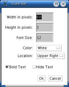
- Photometry Settings
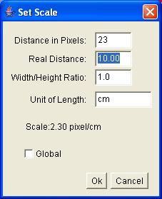
- Set Scale...
- Histogram
- Plot Profile
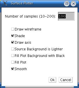
- Surface Plot...
- Radio Spectrum...
- Optical Spectrum...
- Tools
- Calibrate...
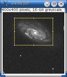
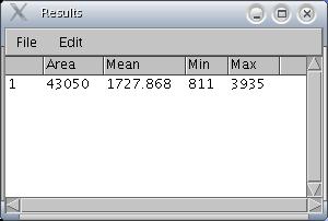
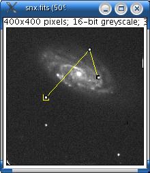
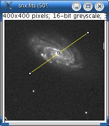
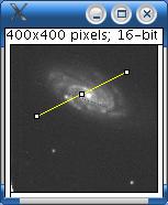
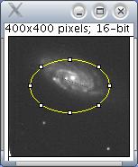
Based on the selection type, calculates and displays either area statistics, line lengths and angles. Area statistics are calculated if there is no selection or if a subregion of the image has been selected using one of the four toolsin the tool bar. Calculates line length and angle if a line selection has been created using one of the three line selection tools
.
Examples :
The width of the columns in the "Results" window can be adjusted by clicking on and dragging the vertical lines that separate the column headings.
Clear Results
Erases the results table and resets the measurement counter.
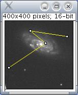
Photometry
Photometry is the determination of the flux of light emitted by a star. It is calculated by correcting the integrated values of the pixels by the value of the sky background. This value can be related to the star intensity selection as shown. Click once to select a subregion of the image where the photometry will be applied.
Example :